Minimum Spanning Trees: Step-by-Step Algorithms and Optimization
In graph theory, finding the most efficient way to connect a set of locations or nodes is a fundamental optimization problem. This is formally solved using a Spanning Tree, which connects all vertices of a graph with the minimum possible number of edges.
When the graph's edges have weights (representing distances, costs, or latencies), we seek the Minimum Spanning Tree (MST) . Formally, given a connected, undirected graph with a weight function , an MST is a subset of edges that spans all vertices without any cycles, such that the total weight is minimized:
The construction of an MST relies heavily on the Cut Property . This mathematical property guarantees that greedy choices lead to a globally optimal solution.
Visualizing a Graph and its MST
Consider the following undirected weighted graph:
By applying an MST algorithm, we extract the optimal cycle-free backbone of the graph with a total cost of 8:
Footnotes
-
Introduction to Algorithms (Wikipedia) - Comprehensive overview of Minimum Spanning Trees, mathematical properties, and basic algorithms. ↩ ↩2
Greedy Algorithms: Prim's and Kruskal's Algorithms
Kruskal's Algorithm
Kruskal's algorithm is an edge-centric Greedy Algorithm . It builds the MST by sorting all edges from lowest weight to highest weight and adding them one by one, provided that the edge does not create a cycle.
To perform cycle detection efficiently, Kruskal's algorithm utilizes a Disjoint-Set Data Structure (also known as Union-Find) . Each vertex starts in its own set. For each edge , we check if and belong to the same set:
- If they do, adding the edge would form a cycle; hence, we discard it.
- If they do not, we add the edge to the MST and merge (union) the two sets.
The total time complexity of Kruskal's algorithm is:
This is because sorting the edges dominates the computational cost, while the subsequent Union-Find operations run in near-linear time , where is the extremely slow-growing inverse Ackermann function .
Footnotes
-
Kruskal's Algorithm (Wikipedia) - Detailed explanation of Kruskal's greedy approach, cycle detection, and Disjoint-Set Union complexity. ↩ ↩2 ↩3
Kruskal's Algorithm Step-by-Step Walkthrough
- 1Step 1
Begin by listing all edges in the graph and sorting them in non-decreasing order of their weights. At the start, each vertex is placed in its own individual disjoint set:
- with weight 1
- with weight 2
- with weight 2
- with weight 3
- with weight 4
- with weight 5
Initial sets: .
- 2Step 2
Select the edge with the smallest weight, which is with weight 1. Check if vertices and belong to the same disjoint set. Since they do not, adding this edge will not form a cycle. We union the sets containing and , and add to our MST.
MST Edges: Active sets: Total weight: 1.
- 3Step 3
Select the next smallest edge, with weight 2. Check if and are in the same disjoint set. Since and , they are in different sets. Add to the MST and union their sets.
MST Edges: Active sets: Total weight: 1 + 2 = 3.
- 4Step 4
Select the next smallest edge, with weight 2. Check if and are in the same disjoint set. Since and , they are in different sets. Add to the MST and union their sets.
MST Edges: Active sets: Total weight: 3 + 2 = 5.
- 5Step 5
Select the next smallest edge, with weight 3. Check if and are in the same disjoint set. Since and , they are in different sets. Add to the MST and union their sets.
MST Edges: Active sets: Total weight: 5 + 3 = 8.
- 6Step 6
The MST now contains edges. All vertices are fully connected in a single set. Any further edge evaluations (like or ) will be rejected because both vertices of those edges already belong to the same set , meaning their addition would form a cycle. The final Minimum Spanning Tree is complete with a total cost of 8.
Handling Disconnected Graphs
If the input graph is not fully connected, Kruskal's algorithm will not yield a single Minimum Spanning Tree. Instead, it will output a Minimum Spanning Forest, which is a collection of MSTs for each individual connected component .
Footnotes
-
Kruskal's Algorithm (Wikipedia) - Detailed explanation of Kruskal's greedy approach, cycle detection, and Disjoint-Set Union complexity. ↩
Prim's Algorithm
Prim's algorithm is a node-centric greedy algorithm . Instead of sorting all edges upfront, it starts with a single arbitrary root vertex and grows the spanning tree one vertex at a time.
At each step, the algorithm chooses the minimum-weight edge that connects a vertex already inside the growing tree to a vertex outside the tree. To do this efficiently, Prim's algorithm maintains a Priority Queue to keep track of the minimum connection costs of all unvisited vertices .
In terms of data representation, the graph is typically modeled using an Adjacency Matrix or an adjacency list.
The time complexity depends on the implementation:
- Adjacency Matrix & linear scan: (optimal for dense graphs) .
- Adjacency List & Binary Heap: .
- Adjacency List & Fibonacci Heap: .
Footnotes
-
Prim's Algorithm (Wikipedia) - In-depth look at Prim's node-growing strategy, priority queue optimization, and complexity. ↩ ↩2 ↩3 ↩4
-
Introduction to Algorithms (Wikipedia) - Comprehensive overview of Minimum Spanning Trees, mathematical properties, and basic algorithms. ↩
Prim's Algorithm Step-by-Step Walkthrough
- 1Step 1
Choose an arbitrary vertex to begin. Let's select vertex . Initialize the set of visited vertices inside the MST as . The set of non-visited vertices is . Track the minimum weight to connect each unvisited vertex to the tree:
- : weight 1 (via )
- : weight 4 (via )
- : (no direct edge from ).
- 2Step 2
Examine the active cut edges crossing from to the unvisited set: with weight 1 and with weight 4. The minimum is . Add to the MST. Update .
Update connection weights for unvisited vertices adjacent to :
- : updated from 4 to 2 (via , which is cheaper)
- : updated from to 3 (via )
- : remains .
- 3Step 3
Examine the active cut edges crossing from to the unvisited set: with weight 4, with weight 2, and with weight 3. The minimum is with weight 2. Add to the MST. Update .
Update connection weights for unvisited vertices adjacent to :
- : updated from to 2 (via )
- : remains 3.
- 4Step 4
Examine the active cut edges crossing from to the unvisited set: with weight 3, with weight 2. The minimum is with weight 2. Add to the MST. Update .
Update connection weights for unvisited vertices adjacent to :
- : remains 3 (since edge has weight 5, which is worse than the existing weight of 3 from ).
- 5Step 5
Examine the active cut edges crossing from to the unvisited set : with weight 3, with weight 5. The minimum is with weight 3. Add to the MST. Update .
All vertices are now included in the tree. The algorithm terminates with a final MST weight of 1 + 2 + 2 + 3 = 8.
Choosing the Right Tool: Prim's vs. Kruskal's
Use Prim's Algorithm (with an adjacency matrix implementation) for dense graphs where because it avoids sorting all edges. Use Kruskal's Algorithm for sparse graphs where because sorting the small number of edges is highly efficient and DSU operations are extremely fast 2.
Footnotes
-
Introduction to Algorithms (Wikipedia) - Comprehensive overview of Minimum Spanning Trees, mathematical properties, and basic algorithms. ↩
-
Kruskal's Algorithm (Wikipedia) - Detailed explanation of Kruskal's greedy approach, cycle detection, and Disjoint-Set Union complexity. ↩
1class DSU:
2    def __init__(self, n):
3        self.parent = list(range(n))
4        self.rank = [0] * n
5
6    def find(self, i):
7        if self.parent[i] == i:
8            return i
9        self.parent[i] = self.find(self.parent[i])  # Path compression
10        return self.parent[i]
11
12    def union(self, i, j):
13        root_i = self.find(i)
14        root_j = self.find(j)
15        if root_i != root_j:
16            if self.rank[root_i] < self.rank[root_j]:
17                self.parent[root_i] = root_j
18            elif self.rank[root_i] > self.rank[root_j]:
19                self.parent[root_j] = root_i
20            else:
21                self.parent[root_j] = root_i
22                self.rank[root_i] += 1
23            return True
24        return False
25
26def kruskal(n, edges):
27    # edges: list of tuples (weight, u, v)
28    edges.sort()
29    dsu = DSU(n)
30    mst = []
31    mst_weight = 0
32    for weight, u, v in edges:
33        if dsu.union(u, v):
34            mst.append((u, v, weight))
35            mst_weight += weight
36            if len(mst) == n - 1:
37                break
38    return mst, mst_weight
Algorithm Performance Comparison (Estimated Operations)
Comparison of theoretical operations for Sparse (E = 2V) vs Dense (E = V^2/2) graphs with V = 100
Historical Evolution of MST Algorithms
Borůvka's Algorithm
1926Otakar Borůvka designed the first known MST algorithm to find an efficient electrical coverage grid for Moravia . It remains highly parallelizable."
Footnotes
-
Introduction to Algorithms (Wikipedia) - Comprehensive overview of Minimum Spanning Trees, mathematical properties, and basic algorithms. ↩
Jarník's Discovery
1930Vojtěch Jarník independently discovered what is now known as Prim's algorithm, focusing on the node-centric growing approach ."
Footnotes
-
Prim's Algorithm (Wikipedia) - In-depth look at Prim's node-growing strategy, priority queue optimization, and complexity. ↩
Kruskal's Algorithm
1956Joseph Kruskal published his edge-centric greedy algorithm, utilizing sorting and disjoint sets to find the minimum spanning forest ."
Footnotes
-
Kruskal's Algorithm (Wikipedia) - Detailed explanation of Kruskal's greedy approach, cycle detection, and Disjoint-Set Union complexity. ↩
Prim's Rediscovery
1957Robert C. Prim independently rediscovered and popularized Jarník's algorithm, establishing its mathematical properties in computer networks ."
Footnotes
-
Prim's Algorithm (Wikipedia) - In-depth look at Prim's node-growing strategy, priority queue optimization, and complexity. ↩
Frequently Asked Questions & Edge Cases
Knowledge Check
Which data structure is most critical for optimizing the cycle-detection step in Kruskal's algorithm?
Explore Related Topics
Dijkstra's Algorithm
Dijkstra's algorithm finds the shortest‑path distances from a single source to all reachable vertices in a weighted graph whose edge weights are non‑negative, using a greedy selection of the minimum‑distance unsettled vertex and edge relaxation.
- Keeps a tentative distance array and a min‑priority queue; extracting the smallest distance finalizes that vertex’s shortest path.
- Correct only for non‑negative edges; negative weights invalidate the greedy invariant.
- With an adjacency‑list and binary heap the time is O((V+E) log V); matrix scans give O(V²) and Fibonacci heaps can achieve O(E + V log V).
- Storing a predecessor array allows reconstruction of actual shortest paths and early termination when a specific target is settled.
- Fundamental in routing, navigation, and as a subroutine in many larger graph algorithms.
Shortest Paths in Unweighted Graphs: Why BFS Wins
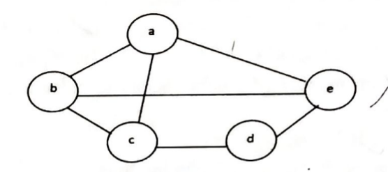
State the graph coloring problem and write the algorithm. Apply backtracking technique to solve the 3-colouring problem for the following graph.